Estimation of the Social Discount Rate (SDR) with Climate Change Uncertainty: The Case of Korea
Abstract
This paper estimates the appropriate social discount rate (SDR) with regard to climate change uncertainty for the Korean economy. First, following Burke et al. (2015)ʹs framework, we measure the marginal economic impact of climate change on the Korean economy focusing on temperature rise. Then, based on this historical relationship, we predict future GDP growth rate according to the climate representative concentration pathway (RCP) and socio‐economic scenarios (SSP) by 2100. Lastly, we estimate the SDR for the Korean economy for the next decade, based on the trajectory of future GDP growth rate.
Overall, taking into consideration that climate uncertainty may be crucial in determining an appropriate SDR for environmental policy appraisal, we find that at given levels of temperature rise, the Korean economy may suffer from global warming relatively more than the rest of the world. Therefore, in the worst‐case scenario, Koreaʹs predicted future GDP growth rate would drastically decline. Consequently, our estimation supports that the appropriate level of SDR calculated based on the Ramsey Rule should decline over time, and even reach negative values depending on the climate scenario.
Keywords:
Climate Change, Social Discount Rate (SDR), Socio‐Economic (SSP) Scenario, RCP Scenario1. Introduction
Over the past decade, huge amounts of literature have shed light on the impact of climate change on various fields (Mendelsohn et al., 1994; Schlenker et al., 2005, 2006; Deschênes and Greenstone, 2007; Schlenker and Roberts, 2009; Welch et al., 2010; Deschênes and Greenstone, 2012; Fisher et al., 2012; Lobell et al., 2013; Chen et al., 2015; Burke and Emerick, 2016). Among the economic literature, there is a burgeoning amount of literature on the climate change impact on GDP growth rates particularly focusing on the temperature rise (Hsiang, 2010; Dell et al., 2012; Deryugina and Hsiang, 2014; Burke et al., 2015). The consensus from these studies is that due to global warming, the total productivity is expected to decline and hence affect the GDP growth rates all over the world as well. If so, how severely will the Korean economy be affected by climate change? Further, at a given level of temperature rise, how much of Korea’s GDP growth rate will decline?
If the GDP loss is relatively large for the Korean economy, then the Korean government should respond to climate change immediately and much more proactively. Furthermore, despite current global efforts for climate mitigation and greenhouse gas reduction, the Korean government should also place emphasis on adaptation policies for the future of the Korean economy.
As part of the movement towards the active response to climate change, estimating the social discount rate (SDR) taking into account climate change is critical. SDR is one of the crucial factors in the policy appraisal process, especially for policies with long-term capital flow. Despite of its importance, a debate on an ‘appropriate’ SDR is still on-going between various prominent scholars (Stern, 2007; Nordhaus, 2007, 2017); variations of the SDR can also be seen by country and sector, demonstrating that there is no universal consensus. In the case of the Korean government, from 2017, the SDR of 4.5% was employed to evaluate the economic values of policies, and additionally, a lower level of SDR is adopted for the policies in the transportation and water sectors that exceed 30 years; however, these rates do not take into account climate change characteristics and uncertainties (KDI, 2008).
In this paper, we estimate the SDR for the Korean economy by taking into consideration the effect of rising temperature. First, we estimate the marginal effect of the rising temperature on the GDP growth rate of Korea between 1960-2010 based on Burke et al. (2015) (hereinafter, BHM)'s framework. Next, based on this historical analysis, we predict future GDP growth rate by 2100, given the scenarios from the socio-economic (SSP) and climate (RCP) conditions. Lastly, we suggest the appropriate level of the SDR for the Korean economy taking into account climate change.
With sufficient controlling of relevant variables, we find that historically, the optimal temperature rate for the Korean economy is actually much lower than what is estimated from the global sample. That means Korea would be severely affected by global warming at the current given rate of predicted temperature rise. If this historical relationship lasts for the next decade, the Korean economy is expected to face negative GDP growth rates by 2100 based on all of the RCP scenarios. These results are based on the 1~3% level of GDP growth rates calculated from the non-climate scenarios (SSP).
Taking into account these climate change paths that affect the GDP growth rate, it is highly likely that the Korean government should employ a much lower rate of SDR than the current rate. Based on the decreasing pattern of GDP growth rate, it is suggested that the SDR should also take form of a declining discount rate (Weitzman, 1998; Groom et al., 2005; Arrow et al., 2014). Our conclusion is consistent with the low level of GDP growth rate cases in past studies for Korea (Lee et al., 2016; Sohn, 2019). This is particularly pertinent in long-term policies like environment policies where the SDR should be lower than the current status quo.
The rest of the paper is organized as follows. In section 2, we provide the conceptual framework of how the SDR and climate change is related in terms of the future GDP growth rate (g). Next, we report our estimation results for g in section 3. In section 4, we demonstrate our main results for the SDR. We then conclude with a summary of the findings in section 5.
2. Conceptual framework
2.1 Social Discount Rate (SDR): Ramsey Rule
Conventionally, the SDR is framed by the Ramsey Rule (Ramsey, 1928) as seen by the following equation:
| (1) |
where ρ is the rate of pure time preference, ζ refers to the elasticity of marginal utility, and g is the future economic growth rate-specifically, the real growth rate of consumption per capita. The first term (ρ) on the right-hand side captures how much today’s society cares for future societies, while the second term (ζ×g) represents the wealth effect, which means the tendency of the economic agents to smooth intergenerational consumption; therefore, if a higher economic growth rate is expected in the future generations, then SDR would also increase.
Among the factors of the SDR, our focus is on g, which is the main source of uncertainty related to climate change (Lewandowsky et al., 2017). Forecasts of the long-run economic growth rate are difficult to determine without a certain level of uncertainty. Moreover, because climate change is an issue of the distant future, the debate centered on the range of its economic impact carries even more layers of uncertainty.
2.2 Relationship Between Economic Growth Rate (g) and Temperature
From the perspective of climate change literature, g can be obtained from a theoretical model (e.g. Nordhaus (2007)), expert survey (e.g. Drupp et al. (2018)), or empirical model (e.g. Christensen et al. (2018)). For empirical studies, temperature and precipitation are the main climate variables in the research (Zhang et al., 2017). Especially, a burgeoning literature has investigated the economic impact of rising temperature (BHM; Colacito et al., 2019; Lee et al., 2016 (hereinafter, LVG); Tang et al., 2018).
As one of the inspiring foundations for this research, BHM investigated the relationship between GDP growth rate and temperature for 166 countries during 1960-2010. With this global sample, they found that the temperature has an inverted-U shaped relationship with the GDP growth rate, with growth peaking at an annual average temperature of 13.06°C. This nonlinear relationship is robust in various specifications; for example, in the analysis of different time period (1960-1989 vs. 1990-2010); income effect (rich vs. poor countries); and industry effect (agricultural vs. non-agricultural). Taking into account for the global non-linear relationship, BHM calculated the “empirical damage function”, which shows the loss of annual average income caused by rises in the temperature. According to their findings, global incomes would be reduced by about 23% by 2100.
3. Estimation of g
This study consists of three parts. First, based on the BHM’s framework specifically for the Korean historical data, we estimate the marginal effect of rising temperature on the economic growth rate from 1960 to 2010. Assuming that the results from this historical estimation represent a steady-state economy, we then compute the future Korean GDP growth rate, g, combined with climate and economic growth projection scenarios. Lastly, by employing the future GDP growth rate obtained from the second stage, we estimate the SDR for the Korean economy by 2100.
3.1 Data and Scenarios
For the historical analysis of 1960-2010 period, we employ a Korean sample from the dataset provided from BHM; the GDP data from the World Bank’s World Development Indicators (WDI); and climate change data (temperature and precipitation) from Matsuura and Willmot (2012). We also use historical temperature data from the Korean Meteorological Administration (KMA), which generate similar results.
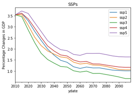
For the projection of g, we rely on the climate and socio-economic scenarios: 3 scenarios of SSPs (SSP2, SSP3 and SSP5) and all of four RCPs. Among the SSP scenarios, SSP2 resembles the median estimation of long-term economic growth rate provided from the Korean government. SSP3 and SSP5 are the scenarios employed by BHM and Lewandowsky et al. (2017), because those scenarios are consistent with the case of high emissions (RCP 8.5). Given these SSP/RCP scenarios, we employ GDP growth rates based on SSPs from OECD, and expected temperature changes in Korea from KMA.
3.2 Historical Analysis
To estimate the relationship between temperature and GDP growth rate, we re-estimate the regression of BHM with a single country sample, specifically Korea. Following BHM, we use second-order polynomials of temperature and precipitation:
| (2) |
where Tt refers to temperature, Pt is precipitation and t is time trends. In our baseline model, we focus on the parameters for quadratic function of temperature (β1 and β2), controlling the precipitation and quadratic time trends.
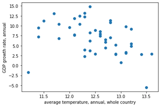
Fig 3 displays an eyeball evidence on the relationship between temperature and GDP growth rate of Korea. Interestingly, both variables have strong linear trends in each of their historical data, but they have nonlinear relationship with each other. For temperature, it shows a stable but rising pattern while the GDP growth rate shows a significantly decreasing pattern. However, as shown in BHM, the Korean economy also demonstrates the inverted-U shaped relationship between the two variables.
Table 2 provides our results from the regression on the Korean sample. The first column shows the overall estimate from BHM based on their global sample and the second is our baseline estimate for Korea. We check with another regression model which includes only linear time trend (column (3)), adding lags of GDP growth rate (column (4) and (5)), and employing other data source from the Penn World Table (PWT) (column (6)). Both the global and Korean sample results show that the nonlinear relationship between temperature and GDP growth rate is significant. Also, for most of the robustness check specifications, the parameters for the quadratic functional form of temperature are significant, even at 1% levels. However, there is a striking difference between the optimal rates of temperature estimated from the two samples; for the Korean case, estimation results show that the economic production is at a maximum of about 11.39°C, which is much lower than that from BHM.
According to results of BHM, Korea can be one of the better-off countries from global warming. Because temperature has a curvilinear relationship with the GDP growth rate, the economy of countries with an annual average temperature lower than 13.06°C can benefit from annual temperature rise. That means South Korea, where the historical annual average temperature is around 12°C (Matsuura and Willmott, 2012; KMA, 2015), can be one of the beneficiaries from global warming. However, based on our estimation, the Korean economy would severely suffer from the effects of global warming. If the optimal temperature for the Korean economy is about 11.3°C, which is already under the historical average annual temperature rate, the rises in temperature in the future will hurt the Korean economy in a nonlinear way; as temperature rises, the loss due to climate change in the Korean economy would thereby escalate.
Our findings are consistent with other studies which indicate that Korea could be one of the worse-off countries from global warming (Puaschunder, 2019). Korea has distinctive four seasons, which means that the negative effect of temperature rising during the hot and humid summer in Korea can be huge (see Colacito et al. (2019) for the seasonal effect analysis). Also, based on the U.S. district level data, (Burke and Tanutama, 2019) found that the optimal temperature rate is lower than 10°C.
3.3 Projection of g
Here, we predict future GDP growth rate by 2100. Combined the optimal temperature estimates with SSP scenarios, we calculate the empirical damage function following BHM. The trajectory of economic production is assumed to be affected by two sources; one is socio-economic activity absent of climate change, and the other is increases in temperature which represent the climate change phenomenon in our paper. Specifically, we calculate gt by combining the GDP growth rate from SSPs (ηt) and that of climate change (δt).
| (3) |
δt is calculated as the empirical damage function h(T), δt=h( ) -h(T) , where refers to the future rate of temperature by 2100, and T refers the historical average rate between 1980 and 2010. , where ΔTRCP is expected increases in temperature for Korea by 2100, according to the RCP scenarios. .
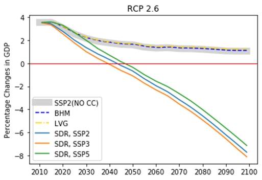
Fig 4 demonstrates the predicted g based on SSP scenarios and three different empirical damage functions: from BHM, LVG, and this paper labelled, SDR. In LVG, the optimal rate of temperature was calculated as 14.24°C, based on the global sample. We employ SSP2 and RCP2.6 for the comparison our baseline model with BHM and LVG specifications, and additionally SSP3 and SSP5 for our model only. The grey area represents GDP growth rates from SSP2 scenario.
As shown in the Fig 4, the level of optimal temperature rate is crucial in calculating future GDP growth rate. Due to the inverted-U shaped relationship, rises in temperature that are below the optimal rate can boost the economy, while oppositely hurt the economy progressively after it reaches temperatures above the optimal rate. Both of the results based on the higher optimal rates from the global samples predict future GDP growth rate which are slightly higher than the SSP growth rate. This indicates that the Korean economy will grow because of the rising temperatures.
However, according to our estimation, these results can drastically shift; even in the most limiting case of RCP 2.6, the Korean economy will suffer severely as temperature rises. The future GDP growth rate is dominated by the damage function of temperature increases, and the results from the different scenarios of SSPs also do not make any sizable changes.
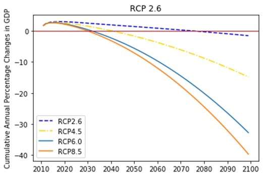
Based on our model, we compute cumulative annual GDP growth rates, the one of SDR components, according to RCP scenarios. Combined with the lower level of optimal rate and the nonlinear relationship, the more the temperature rises, the bigger the economic losses from climate change is expected.
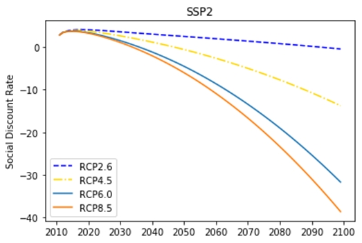
Fig 5 displays the cumulative GDP growth rate in different RCP scenarios. When we consider RCP 8.5 scenarios, the economic loss can be as catastrophic as -40 percent. Furthermore, for all of the RCP scenarios, the Korean economy would suffer from the rising temperature by 2100.
These shocking results come from two sources; the nonlinearity and the level of optimal temperature rate. Taking into account the nonlinearity relationship generates huge economic costs from climate change, compared to the damage function proposed by the Integrated Assessment Models (IAMs). Since IAMs employ a linear function of temperature and GDP relationship, the cost of rising temperature would be relatively limited. In contrast, the empirical analysis in BHM from the global samples provide evidence for substantial amount of the global economic loss. In this paper we demonstrate that this conclusion obtained from the global sample estimation also can be applied to the Korean economy. Moreover, because our result shows that the lower rate of temperature is optimal for the Korean economy, accounting for the nonlinearity relationship generates even more severe damage function for the Korean economy.
4. Estimation of SDR
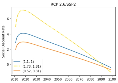
Lastly, we estimate the SDR for the Korean economy based on the previous results. First, we calculate the SDR for RCP2.6 and SSP2 cases. Given the framework of Ramsey Rule, we calculate the forward rate of SDR (see e.g., (Lewandowsky et al., 2017)). For other parameters in SDR, ρ and ζ, we employ a three prong approach from past studies of Korean SDR estimations (Lee et al., 2016; Kim, 2015; Sohn, 2019): middle (1.1, 1), high (1.73, 1.81) and low (0.52, 0.81). The numbers in the parenthesis in the legend (Fig 6) refers to the values of ρ (first) and ζ (second) from past studies. Fig 6 shows the estimated SDRs for the Korean economy. All of the SDRs share similar patterns where they decrease over the horizon, and even for the case of RCP 2.6, become negative by 2100. Because the decreasing pattern of SDR arises from the trajectory of g which falls over time, SDR declines remarkably when we consider other RCP scenarios (Fig 7). Based on the decreasing pattern of the GDP growth rate, it is suggested that the SDR should also take form of a declining discount rate (Weitzman, 1998). In sum, our conclusion is consistent with past studies that estimate the SDR for Korea with low level of future GDP growth rate (Lee et al., 2016; Sohn, 2019).
5. Conclusion
In this paper, we estimate the SDR for the Korean economy, based on the prediction of future GDP growth rate by combining historical estimation adapted from BHM for the Korean case, with the future scenarios of climate and socio-economic behaviors.
We propose that Korea can be quite vulnerable to impacts of climate change and that the Korean economy would be hurt relatively more than other countries at a given magnitude of temperature rising, because it has a lower level of overall optimal temperature rate. These empirical findings can be applied in the calculation of the SDR, which is a crucial factor for policy appraisal. Thus, according to our findings, the SDR should be the set at a substantially low level, and even reach negative values for long-term policies by 2100.
Additionally, the negative impact of rising temperature would be exaggerated in the future, as the magnitude of climate change for Korea can be larger. South Korea is geographically located where global warming is severe (IPCC, 2013). In the same light, the temperature of South Korea has risen by 1.7°C, which is more than twice the global average of 0.7°C (Park, 2015). That means without significant reduction of CO2, we should alter our prediction that future generations will be richer than the current generation, as Korea is expected to become warmer. Furthermore, the Korean government should also place emphasis on climate adaptation policies to its economic structure, in order to reduce the magnitude of GDP loss from global warming.
We must recognize that when focusing on the historical relationship, empirical results from BHM and this paper, also have several caveats: although we employ several future scenarios from the IPCC to address this issue, a limit to incorporating all future changes and other source of uncertainties still remains (Lewandowsky et al., 2017). Additionally, other than the historical analysis, there are some debates about the BHM’s estimation results (Rosen, 2019; Diffenbaugh, 2019). Therefore, our conclusion should be further adapted according to the consensus derived from these debates in the future.
Acknowledgments
This work is supported by Korea Environment Industry & Technology Institute (KEITI) through Climate Change R&D Program, funded by Korea Ministry of Environment (MOE) (2018001310003).
We would also like to express our gratitude to M. Burke, S. Hsiang and E. Miguel for publicly sharing their model and findings that was the inspiration for our paper. Lastly, we would like to thank the participants of the Korea Resource Economics Association June 2019 conference and the Korea Society of Climate Change June 2019 conference for their useful comments and suggestions.
References
-
Arrow KJ, Cropper ML, Gollier C, Groom B, Heal GM, Newell RG, Nordhaus WD, Pindyck RS, Pizer WA, Portney PR. 2014. Should governments use a declining discount rate in project analysis? Rev Environ Econ Policy. 8 (2): 145-163.
[https://doi.org/10.1093/reep/reu008]

-
Burke M, Emerick K. 2016. Adaptation to climate change: Evidence from US agriculture. Am Econ J Econ Policy. 8 (3): 106-140.
[https://doi.org/10.1257/pol.20130025]

-
Burke M, Hsiang SM, Miguel E. 2015. Global non-linear effect of temperature on economic production. Nature. 527 (7577): 235-239.
[https://doi.org/10.1038/nature15725]

-
Burke M, Tanutama V. 2019. Climatic Constraints on Aggregate Economic Output. National Bureau of Economic Research.
[https://doi.org/10.3386/w25779]

-
Chen Y, Li Z, Fan Y, Wang H, Deng H. 2015. Progress and prospects of climate change impacts on hydrology in the arid region of northwest China. Environ Res. 139: 11-19.
[https://doi.org/10.1016/j.envres.2014.12.029]

-
Christensen, P, K Gillingham, and W Nordhaus. 2018. “Uncertainty in Forecasts of Long-Run Economic Growth.” (to 2100).
[https://doi.org/10.1073/pnas.1713628115]

-
Colacito R, Hoffmann B, Phan T. 2019. Temperature and Growth: A Panel Analysis of the United States. J Money, Credit Bank. 51 (2-3): 313-368.
[https://doi.org/10.1111/jmcb.12574]

-
Dell M, Jones BF, Olken BA. 2012. Temperature shocks and economic growth: Evidence from the last half century. Am Econ J Macroecon. 4 (3): 66-95.
[https://doi.org/10.1257/mac.4.3.66]

-
Deryugina T, Hsiang SM. 2014. Does the environment still matter? Daily temperature and income in the United States. National Bureau of Economic Research.
[https://doi.org/10.3386/w20750]

-
Deschênes O, Greenstone M. 2012. The economic impacts of climate change: evidence from agricultural output and random fluctuations in weather: reply. Am Econ Rev. 102 (7): 3761-3773.
[https://doi.org/10.1257/aer.102.7.3761]

-
Deschênes O, Greenstone M. 2007. The economic impacts of climate change: evidence from agricultural output and random fluctuations in weather. Am Econ Rev. 97 (1): 354-385.
[https://doi.org/10.1257/aer.97.1.354]

-
Diffenbaugh NS, Burke M. 2019. Reply to Rosen: Temperature–growth relationship is robust. Proc Natl Acad Sci. 116 (33): 16171-16172.
[https://doi.org/10.1073/pnas.1908772116]

-
Drupp MA, Freeman MC, Groom B, Nesje F. 2018. Discounting disentangled. Am Econ J Econ Policy. 10 (4): 109-134.
[https://doi.org/10.1257/pol.20160240]

-
Fisher AC, Hanemann WM, Roberts MJ, Schlenker W. 2012. The economic impacts of climate change: evidence from agricultural output and random fluctuations in weather: comment. Am Econ Rev. 102 (7): 3749-3760.
[https://doi.org/10.1257/aer.102.7.3749]

-
Groom B, Hepburn C, Koundouri P, Pearce D. 2005. Declining discount rates: the long and the short of it. Environ Resour Econ. 32 (4): 445-493.
[https://doi.org/10.1007/s10640-005-4681-y]

-
Hsiang SM. 2010. Temperatures and cyclones strongly associated with economic production in the Caribbean and Central America. Proc Natl Acad Sci. 107 (35): 15367-15372.
[https://doi.org/10.1073/pnas.1009510107]

- IPCC. 2013. Climate Change 2013: The Physical Science Basis. Contribution of Working Group I to the Fifth Assessment Report of the Intergovernmental Panel on Climate Change. Stocker TF, Qin D, Plattner G-K, Tignor M, Allen SK, Boschung J, Nauels A, Xia Y, Bex V, Midgely PM, editors. Cambridge, United Kingdom and New York, NY, USA: Cambridge University Press.
-
Kim SK. 2015. The Effect of Social Discount Rate Manipulation on the Economic Feasibility Tests: Focusing on the Environmental Public Investment Projects. J Environ Policy. 12 (4): 71-92.
[https://doi.org/10.17330/joep.12.4.201312.71]

- Korea Development Institute (KDI). Revised and Supplementary General Guidelines for Conducting Preliminary Feasibility Studies (5th edition). 2008.
- Korea Meteorological Administration (KMA). Production of Fine-Scale Climate Change Data over the Korean Peninsula Using RCP Scenarios. 2015.
- Lee J, Kim S, Kim G. 2016. An Expert Survey on the Social Discount Rate in Korea. Korea Energy Econ Inst. 15 (1): 207-237. (in Korean with English abstract)
- Lee M, Villaruel ML, Gaspar RE. 2016. Effects of Temperature Shocks on Economic Growth and Welfare in Asia. Asian Development Bank ADB Economics Working Paper Series. https://econpapers.repec.org/, RePEc:ris:adbewp:0501.
-
Lewandowsky S, Freeman MC, Mann ME. 2017. Harnessing the uncertainty monster: Putting quantitative constraints on the intergenerational social discount rate. Glob Planet Change. 156: 155-166.
[https://doi.org/10.1016/j.gloplacha.2017.03.007]

-
Lobell DB, Baldos ULC, Hertel TW. 2013. Climate adaptation as mitigation: the case of agricultural investments. Environ Res Lett. 8 (1): 15012.
[https://doi.org/10.1088/1748-9326/8/1/015012]

- Matsuura K, Willmott CJ. 2012. Terrestrial precipitation: 1900-2010 gridded monthly time series. WWW Doc URL http//climategeogudeledu/~Clim.2, .
- Mendelsohn R, Nordhaus WD, Shaw D. 1994. The Impact of Global Warming on Agriculture: A Ricardian Analysis. Am Econ Rev. 84 (4): 753-771.
-
Nordhaus WD. 2007. A review of the Stern review on the economics of climate change. J Econ Lit. 45 (3): 686-702.
[https://doi.org/10.1257/jel.45.3.686]

-
Nordhaus WD. 2017. Revisiting the social cost of carbon. Proc Natl Acad Sci. 114 (7): 1518-1523.
[https://doi.org/10.1073/pnas.1609244114]

- Park CY. 2015. The classification of extreme climate events in the Republic of Korea, J Korean Assoc Regional Geographers 21 (2): 394-410. (in Korean with English abstract)
-
Puaschunder JM. 2019. Future Climate Wealth of Nations’ Winners and Losers. Available SSRN 3332544.
[https://doi.org/10.2139/ssrn.3332544]

-
Ramsey FP. 1928. A mathematical theory of saving. Econ J. 38 (152): 543-559.
[https://doi.org/10.2307/2224098]

-
Rosen RA. 2019. Temperature impact on GDP growth is overestimated. Proc Natl Acad Sci. 116 (33): 16170.
[https://doi.org/10.1073/pnas.1908081116]

-
Schlenker W, Hanemann WM, Fisher AC. 2005. Will US agriculture really benefit from global warming? Accounting for irrigation in the hedonic approach. Am Econ Rev. 95 (1): 395-406.
[https://doi.org/10.1257/0002828053828455]

-
Schlenker W, Hanemann WM, Fisher AC. 2006. The impact of global warming on US agriculture: an econometric analysis of optimal growing conditions. Rev Econ Stat. 88 (1): 113-125.
[https://doi.org/10.1162/003465306775565684]

-
Schlenker W, Roberts MJ. 2009. Nonlinear temperature effects indicate severe damages to US crop yields under climate change. Proc Natl Acad Sci. 106 (37): 15594-15598.
[https://doi.org/10.1073/pnas.0906865106]

-
Sohn W-S. 2019. Discount rate and the social cost of carbon dioxide: a Korean forecast. Appl Econ. 51 (32): 1-15.
[https://doi.org/10.1080/00036846.2019.1581907]

-
Stern N. 2007. The Economics of Climate Change. The Stern Review. Cambridge, New York: Cambridge University Press.
[https://doi.org/10.1017/CBO9780511817434]

-
Tang K, Allen MR, Pretis F, Schwarz M, Haustein K. 2018. Uncertain impacts on economic growth when stabilizing global temperatures at 1.5°C or 2°C warming. Philos Trans R Soc A Math Phys Eng Sci. 376 (2119): 20160460.
[https://doi.org/10.1098/rsta.2016.0460]

-
Weitzman ML. 1998. Why the far-distant future should be discounted at its lowest possible rate. J Environ Econ Manage. 36 (3): 201-208.
[https://doi.org/10.1006/jeem.1998.1052]

-
Welch JR, Vincent JR, Auffhammer M, Moya PF, Dobermann A, Dawe D. 2010. Rice yields in tropical/subtropical Asia exhibit large but opposing sensitivities to minimum and maximum temperatures. Proc Natl Acad Sci. 107 (33): 14562-14567.
[https://doi.org/10.1073/pnas.1001222107]

- World Bank Group. World Development Indicators. 2017.
-
Zhang P, Zhang J, Chen M. 2017. Economic impacts of climate change on agriculture: The importance of additional climatic variables other than temperature and precipitation. J Environ Econ Manage. 83: 8-31.
[https://doi.org/10.1016/j.jeem.2016.12.001]


